
Docs · guide
How to highlight duplicates in Excel, and what the rule counts
By Alberto Gulotta · Updated · 19 min read
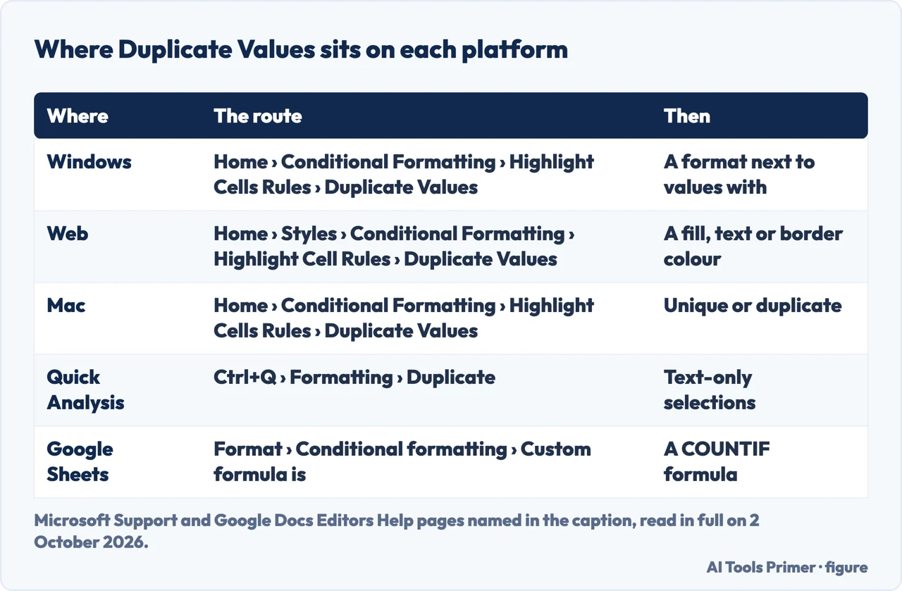
The short answer to how to highlight duplicates in Excel: select the cells, then Home › Conditional Formatting › Highlight Cells Rules › Duplicate Values, and pick a format. That is Microsoft’s route for Windows; its Web tab says Highlight Cell Rules, and its Mac pages add a step to the advanced rule. Clear Rules takes the colour off again.
| Where | The route | What comes next | Page read |
|---|---|---|---|
| Excel on Windows | Home › Conditional Formatting › Highlight Cells Rules › Duplicate Values | Pick a format in the box next to values with, then OK | Find and remove duplicates; five products, and no Mac |
| Excel for the web | Home › Styles › Conditional Formatting › Highlight Cell Rules › Duplicate Values | Enter the values and select a fill, text or border colour | Use conditional formatting to highlight information, Web tab |
| Excel for Mac | Home › Conditional Formatting › Highlight Cells Rules › Duplicate Values | Next to values in the selected range, unique or duplicate | Highlight patterns and trends with conditional formatting in Excel for Mac; Mac only |
| Quick Analysis, on Windows | The Quick Analysis button or Ctrl+Q › Formatting › Duplicate | Offered when the selection holds text only | Use conditional formatting to highlight information, Windows tab |
| Google Sheets | Format › Conditional formatting › Custom formula is | =COUNTIF($A$1:$A$100,A1)>1 for cells A1 to A100 |
Use conditional formatting rules in Google Sheets |
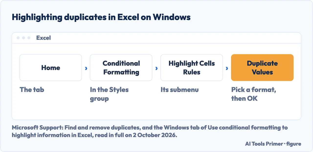
- Select the cells you want to check. A column, a range or a table. The Windows tab of Microsoft’s page on unique and duplicate values allows a PivotTable report too, with one exception, printed on the page Find and remove duplicates: “Excel can’t highlight duplicates in the Values area of a PivotTable report.”
- Open Duplicate Values. On the Home tab, select Conditional Formatting, then Highlight Cells Rules, then Duplicate Values. Microsoft’s page Find and remove duplicates prints this route for five products, and no Mac.
- Pick a format and select OK. In the box next to values with, choose the formatting for the duplicate values. The advanced version of the rule, under Manage Rules and New Rule, is Format only unique or duplicate values, with unique or duplicate in its Format all list.
- Read what is coloured before acting on it. Microsoft gives the reason for the whole exercise: “That way you can review the duplicates and decide if you want to remove them.” Each cell whose value repeats in the selection takes the colour, the first one included; that reading is ours. In Microsoft’s Mac example of the formula rule below, the cities with more than one instance are Seattle and Spokane.
- Take the rule off when you are done. On the Windows tab of Use conditional formatting to highlight information: Home, Conditional Formatting, Clear Rules, Clear Rules from Entire Sheet. Microsoft’s Mac page describes conditional formatting as changing the appearance of cells, so the values stay as they were; that conclusion is ours.
The same rule on the web, on a Mac, and with Quick Analysis
“In the Style list, choose Classic”
That is the step a Mac adds to the advanced rule, on Microsoft’s Mac-only page Filter for or remove duplicate values: New Rule, Classic in the Style list, then Format only unique or duplicate values. For the quick rule the Mac pages print the Windows names. Highlight patterns and trends: on the Home tab select Conditional Formatting, point to Highlight Cells Rules, select Duplicate Values, and next to values in the selected range choose unique or duplicate. The page on filtering then has you choose the options in the New Formatting Rule dialog box. Both pages list Excel for Microsoft 365 for Mac, Excel 2024 for Mac and Excel 2021 for Mac.
Excel for the web. The Web tab of Use conditional formatting to highlight information prints Home, Styles, Conditional Formatting, Highlight Cell Rules, Duplicate Values, with Cell where the Windows menu says Cells. Then you enter the values you want to use and select a fill, text or border colour. On the web the rules live in a Conditional Formatting task pane, which Manage Rules opens. The Web tab of the page on unique and duplicate values covers removing them and nothing else.
Quick Analysis, on Windows. Select the data, then the Quick Analysis button at the lower-right corner of the selection, or press Ctrl+Q. On its Formatting tab, the Windows tab says, Duplicate and Unique are offered when the selection contains only text; for numbers, or numbers and text, the list is Data Bars, Colors, Icon Sets, Greater, Top 10% and Clear. So a column of numbers goes through the ribbon; that advice is ours.
A key sequence. Wall Street Prep, a training company whose guide was read for this one, gives Alt, H, L, H, D, each key pressed on its own, for the Windows ribbon. No Microsoft page read for this guide prints that sequence.
A formula rule: COUNTIF for one column, COUNTIFS for whole rows
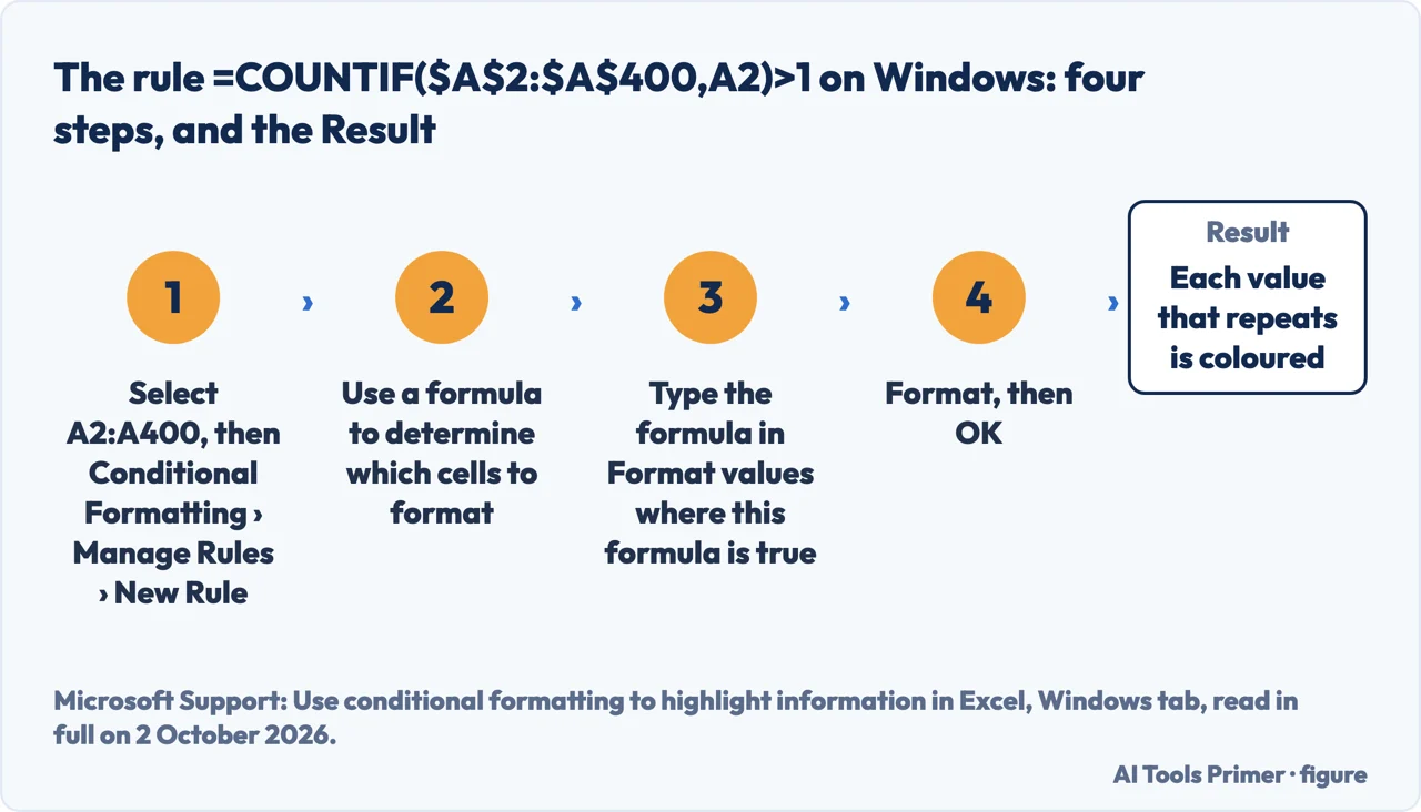
Microsoft prints the formula itself, in a tip on the Windows tab: for duplicates in
A2:A400, a COUNTIF formula rule with =COUNTIF($A$2:$A$400,A2)>1, where the
tip has a space before the 1. The reason it gives is narrow. With a proofing
language such as Japanese, Duplicate Values treats halfwidth and fullwidth characters as the
same, and to tell them apart it points to the formula. The Mac page on formulas uses the same pattern,
=COUNTIF($D$2:$D$11,D2)>1, on a list of ten cities, where it marks Seattle and
Spokane, and Google’s page prints it for Sheets.
Where to type it. On Windows: Home, Conditional Formatting, Manage Rules, New Rule, Use a formula to determine which cells to format, then the formula in Format values where this formula is true, and Format. On the web, Formula in the Rule Type list. On a Mac: New Rule, Classic in the Style box, Use a formula to determine which cells to format, and Customised format in the Format with box. The range carries dollar signs and the single cell does not, so each cell is counted against the whole range; Wall Street Prep explains the anchors the same way. More on references is on the page on conditional formatting with a formula.
Rows that repeat across columns. COUNTIF takes one criterion, and its page says to use
COUNTIFS for more. To mark rows whose values in both A and B repeat, select A2:B400 and use
=COUNTIFS($A$2:$A$400,$A2,$B$2:$B$400,$B2)>1. That formula is ours, written to
the syntax on Microsoft’s COUNTIFS page, and it has not been tested in Excel for this
guide; Acuity Training, another training company read for this guide, prints the same pattern with =2, which marks
the rows that appear exactly twice. The dollar before A and B keeps every cell of a row on the same test, so the whole
row takes the colour; that reading is ours. Excel University, a third, joins the
columns into a helper column with CONCAT instead.
Every repeat but the first. Excel University’s
=COUNTIF($B$2:$B2,$B2)>1 counts from the top of the list down to the current
row, so the first occurrence stays white and the later ones are marked. That method is
theirs, not Microsoft’s.
What Excel counts as a duplicate, and where the rule does not reach
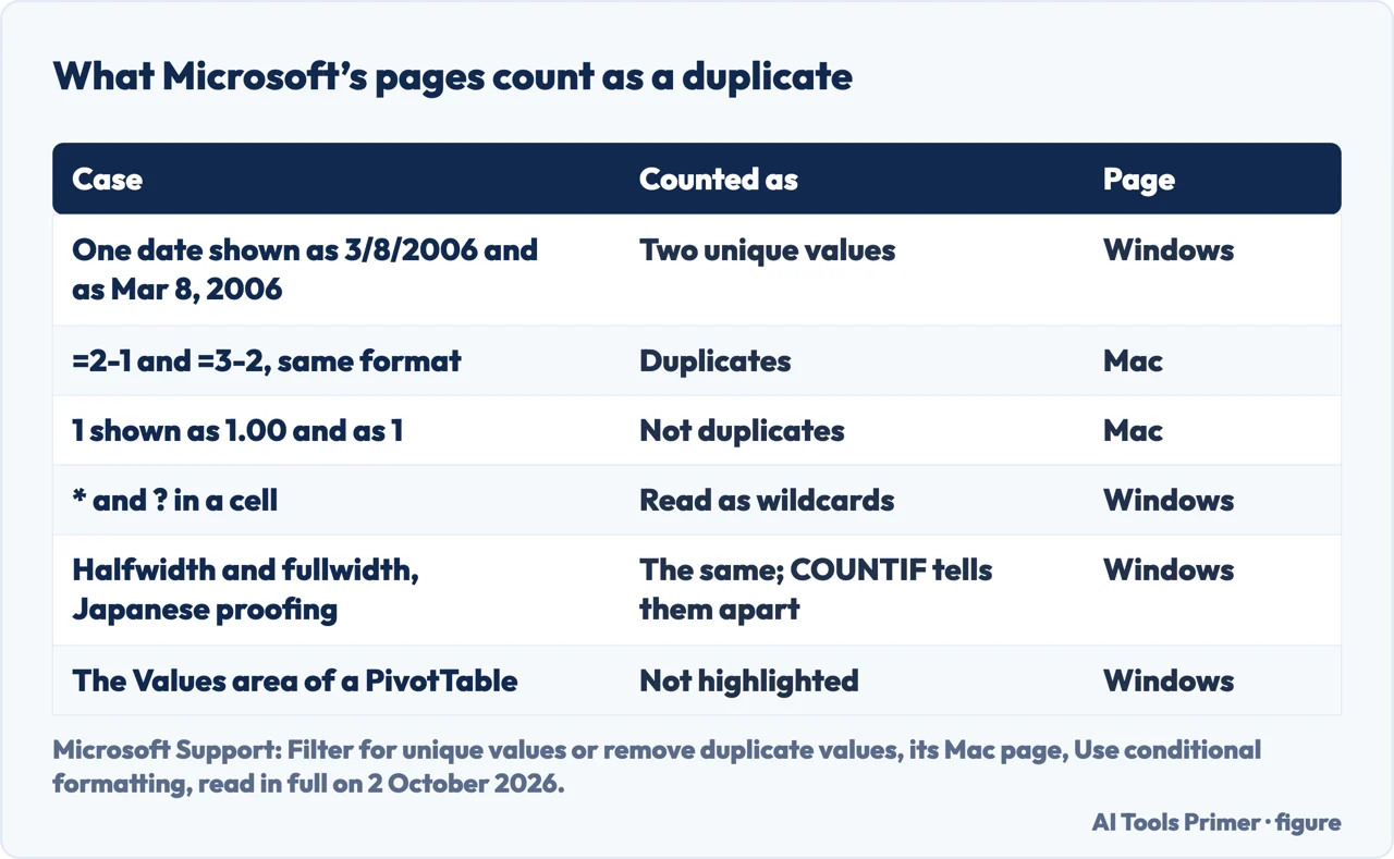
“A comparison of duplicate values depends on what appears in the cell—not the underlying value stored in the cell.”
That is Microsoft’s page on unique and duplicate values, for five products and no Mac, and its example is a date shown as 3/8/2006 in one cell and Mar 8, 2006 in another: two unique values. The Mac page says the same with 12/8/2017 and Dec 8, 2017, and adds two cases. Formulas that differ and return the same value, =2-1 and =3-2, are duplicates when the format is the same; and “If the same value is formatted using different number formats, they are not considered duplicates.” Both pages write this in their opening, before the sections on filtering, removing and conditional formatting; that it holds for the highlight rule too is this guide’s reading.
Asterisks and question marks. The Windows tab of Use conditional formatting to highlight information: the Unique and Duplicate Values rules read * and ? as wildcard characters, even when they are used in a formula in a cell. So a cell holding a* can match cells that are not equal to it; that consequence is ours, and Acuity Training reports the case of a question mark. COUNTIF reads wildcards in its criteria too, by its own page, which says a tilde in front finds an actual question mark or asterisk. No page read for this guide applies the tilde to a duplicate rule.
Capitals. The COUNTIF page: “Criteria aren’t case sensitive.” So Apple and apple count as one value in the formula rule, by this guide’s reading. No Microsoft page read for this guide says whether Duplicate Values tells them apart; Acuity Training writes that neither the rule nor COUNTIF does.
Spaces and long text. The COUNTIF page warns that leading and trailing spaces, mixed straight and curly quotation marks, or nonprinting characters can make it return an unexpected value, and names CLEAN and TRIM; the guide on removing spaces in Excel covers both. It also returns incorrect results for strings longer than 255 characters.
A PivotTable. The Values area is out of reach: the Windows tab says you cannot format such fields by unique or duplicate values. Other cells of a pivot table are in the list of what you can select.
Taking the rule off again
Clearing a rule takes the colour away and, by this guide’s reading, leaves the values as they were.
- Windows
- Home, Conditional Formatting, Clear Rules, Clear Rules from Entire Sheet. For a range, the Windows tab selects the cells and uses the Quick Analysis Lens button and Clear Format. Go To Special, Conditional formats and Same find every cell that carries the same rule.
- The web
- Home, Styles, Conditional Formatting, Clear Rules, then Clear Rules from Selected Cells or Clear Rules from Entire Sheet. In the task pane, the delete button on a rule removes that rule, and Delete All Rules removes every rule in scope.
- Mac
- Select the cells, select Conditional Formatting on the Home tab, point to Clear Rules and choose. Edit, Clear, Formats removes conditional formats and every other cell format.
- Google Sheets
- Point to the rule and click Remove.
The same job in Google Sheets. Google’s page Use conditional formatting rules in Google Sheets gives it as its first example of a custom formula: select A1 to A100, Format, Conditional formatting, Custom formula is, and =COUNTIF($A$1:$A$100,A1)>1. Wildcards there belong to the Text contains and Text does not contain fields. What Sheets counts as a duplicate when it deletes them is on the page on duplicates in Google Sheets.
When the repeats should go. Deleting them is a different command, Data › Data Tools › Remove Duplicates, which Microsoft says deletes permanently and advises running on a copy. The steps, and which row it keeps, are on the page on removing duplicates in Excel.
Where to start
Five ways in.
- “Just give me the steps.”
- Five steps on Windows — the steps on windows
- “My menu says something else.”
- The web, a Mac, Quick Analysis — the route on the web and on a mac
- “I need whole rows, not cells.”
- COUNTIF and COUNTIFS — a formula rule with countif
- “Two cells look alike and stay white.”
- Formats, wildcards, capitals — what excel counts as a duplicate
- “How do I get rid of the colour?”
- Clear Rules, platform by platform — taking the rule off again
Deleting the repeats, and the same job elsewhere
Removing duplicates, the Google Sheets version and formula rules each have a guide of their own.
Cleaning the column before comparing it
Stray spaces, cells that are not blank and pivot tables each have a guide of their own.
Questions people also ask
How do I find duplicates in Excel without removing them?
Highlight them: Home, Conditional Formatting, Highlight Cells Rules, Duplicate Values colours the repeats so that you can review them, Microsoft says, before deciding whether to remove them. Microsoft also prints Data, Sort & Filter, Advanced with Unique records only; its page says the duplicate values are then only hidden temporarily.
Is there an Excel formula to find duplicates?
Yes. Microsoft gives =COUNTIF($A$2:$A$400,A2)>1 for a conditional formatting rule on A2:A400, with the rule type Use a formula to determine which cells to format. Typed into a column beside the data, COUNTIF($A$2:$A$400,A2) returns how many times each value appears; that use outside a rule is this guide’s suggestion.
Why isn’t Excel highlighting duplicate values?
Three notes in Microsoft’s pages fit: the comparison uses what the cell shows, so one date in two formats is two values; the Values area of a PivotTable cannot be highlighted; and the rule reads * and ? as wildcards. Reading them as the cause, and checking the range the rule applies to, is this guide’s advice.
What is the fastest way to remove duplicates in Excel?
This guide has not timed the routes. Microsoft’s command is Data, Data Tools, Remove Duplicates, and its page says the deletion is permanent and suggests copying the data to another worksheet first. Microsoft suggests filtering or conditionally formatting the unique values first, to confirm the result; the steps are on the page on removing duplicates in Excel.
Not covered here. It does not cover macros. Microsoft’s VBA reference has FormatConditions.AddUniqueValues, which returns a UniqueValues object, and its DupeUnique property takes xlDuplicate (1) or xlUnique (0); this guide prints no macro and has tested none.
Nor does it cover giving each repeated value a colour of its own.
Each route taken from a Microsoft page names its tab or its platform; the Applies To lines are in the Sources.
Sources
- Microsoft Support — Find and remove duplicates: Home, Conditional Formatting, Highlight Cells Rules, Duplicate Values, the box next to values with, the note on the Values area of a PivotTable report, and the sentence on reviewing the duplicates before removing them. Applies to Excel for Microsoft 365, Excel 2024, Excel 2021, Excel 2019 and Excel 2016 — five products, and no Mac — support.microsoft.com, read 2 October 2026.
- Microsoft Support — Filter for unique values or remove duplicate values: the comparison of what appears in the cell, with the 3/8/2006 example, the COUNTIF tip for halfwidth and fullwidth characters, the quick and advanced formatting on its Windows tab, the Advanced filter that hides duplicates temporarily, and a Web tab that covers removing them only. Applies to Excel for Microsoft 365, Excel 2024, Excel 2021, Excel 2019 and Excel 2016 — five products, and no Mac — support.microsoft.com, read 2 October 2026.
- Microsoft Support — Use conditional formatting to highlight information in Excel: on its Windows tab, Format only unique or duplicate values, the wildcard note, the COUNTIF tip, the PivotTable note, Quick Analysis and Ctrl+Q, the formula rule type and Clear Rules; on its Web tab, Highlight Cell Rules, Duplicate Values, the task pane, the Formula rule type and Clear Rules. Applies to Excel for Microsoft 365, Excel 2024, Excel 2021, Excel 2019 and Excel 2016 — five products, and no Mac — support.microsoft.com, read 2 October 2026.
- Microsoft Support — Highlight patterns and trends with conditional formatting in Excel for Mac: Highlight Cells Rules, Duplicate Values, unique or duplicate next to values in the selected range, Clear Rules, and Edit, Clear, Formats. Applies to Excel for Microsoft 365 for Mac, Excel 2024 for Mac and Excel 2021 for Mac — Mac only — support.microsoft.com, read 2 October 2026.
- Microsoft Support — Filter for or remove duplicate values, for Mac: the value displayed in the cell, the 12/8/2017 example, the cases of =2-1 and =3-2 and of 1.00 and 1, the New Formatting Rule dialog box, and Classic in the Style list for the advanced rule. Applies to Excel for Microsoft 365 for Mac, Excel 2024 for Mac and Excel 2021 for Mac — Mac only — support.microsoft.com, read 2 October 2026.
- Microsoft Support — Use a formula to apply conditional formatting in Excel for Mac: Classic in the Style box, Use a formula to determine which cells to format, Customised format, and =COUNTIF($D$2:$D$11,D2)>1 on a list of ten cities. Applies to Excel for Microsoft 365 for Mac, Excel 2024, Excel 2024 for Mac and Excel 2021 for Mac — four entries — support.microsoft.com, read 2 October 2026.
- Microsoft Support — Use the COUNTIF function in Microsoft Excel: one criterion and COUNTIFS for more, wildcards and the tilde, criteria that are not case sensitive, strings longer than 255 characters, and spaces and nonprinting characters. Applies to Excel for Microsoft 365, Excel 2024 and Excel 2021, each with its Mac version — six products — support.microsoft.com, read 2 October 2026.
- Microsoft Support — COUNTIFS function: the syntax with criteria_range1, criteria1 and further pairs, up to 127, ranges of the same size. Applies to Excel for Microsoft 365, Excel 2024 and Excel 2021, each with its Mac version, Excel 2019, Excel 2016 and Excel Web App — nine entries — support.microsoft.com, read 2 October 2026.
- Microsoft Learn — FormatConditions.AddUniqueValues method (Excel): returns a UniqueValues object. No Applies To line — learn.microsoft.com, read 2 October 2026.
- Microsoft Learn — UniqueValues object (Excel): the DupeUnique property. No Applies To line — learn.microsoft.com, read 2 October 2026.
- Microsoft Learn — XlDupeUnique enumeration (Excel): xlDuplicate 1 and xlUnique 0. No Applies To line — learn.microsoft.com, read 2 October 2026.
- Google Docs Editors Help — Use conditional formatting rules in Google Sheets: Format, Conditional formatting, Custom formula is, =COUNTIF($A$1:$A$100,A1)>1 as Example 1 of its custom formulas, wildcards in the Text contains fields, and Remove. The Computer version of the page — support.google.com, read 2 October 2026.
- Wall Street Prep — Highlight Duplicate Values in Excel, updated 6 December 2023, the first search result on 2 October 2026, read for this guide: the key sequence Alt, H, L, H, D and the anchors of the COUNTIF rule. A company that sells financial training — www.wallstreetprep.com, read 2 October 2026.
- Acuity Training — Ultimate Guide: Highlighting Duplicate Values Excel, dated 26 February 2024 and updated 19 June 2026, the fourth search result on 2 October 2026, read for this guide: the COUNTIFS pattern with =2, the question mark, and capitals. A company that sells training courses — www.acuitytraining.co.uk, read 2 October 2026.
- Excel University — How to Highlight Duplicates in Excel, dated 26 July 2022, the fifth search result on 2 October 2026, read for this guide: =COUNTIF($B$2:$B2,$B2)>1 for every repeat but the first, and the helper column with CONCAT. A company that sells Excel training — www.excel-university.com, read 2 October 2026.
Written by Alberto Gulotta
Founder and editor of AI Tools Primer, writing from Palermo, Italy. Thirty-five years of taking computers apart, starting with a Commodore 64 — the long version is on the about page.
Something wrong on this page? Write to aitoolsprimer@gmail.com and it gets fixed.
Written on 2 October 2026.
Independence and limits
No affiliate links and no paid placements anywhere on this site. Nobody pays to appear here, and no company has seen this page before you did.
This is general information, not professional advice. Where a page touches money, health, safety or the law, it names its source and the date it was read — and your situation may still differ. See the privacy page and the cookie policy.