Docs · guide

Excel conditional formatting formula: what the reference decides

By Alberto Gulotta · Updated 24 September 2026 · 13 min read

An Excel conditional formatting formula is a rule you write instead of picking one from the list: Home, Conditional Formatting, New Rule, then Use a formula to determine which cells to format. It must start with an equals sign and come out true or false. What decides whether it colours the right cells is the dollar signs.

What a formula rule has to satisfy, in Microsoft’s own words
The requirement	What it means in practice	Source
It starts with `=`	“You have to start the formula with an equal sign (=)”. Exceljet adds what happens without it: Excel turns the rule into text.	Microsoft
It returns TRUE or FALSE	“the formula must return a logical value of TRUE (1) or FALSE (0)”.	Microsoft
It is written for one cell	Write it as though it sat in the top-left cell of the selection; Excel then copies it across the rest.	Exceljet
Its references are locked on purpose	Clicking a cell to build the formula gives you an absolute reference. Relative is what makes the rule move down a column.	Microsoft

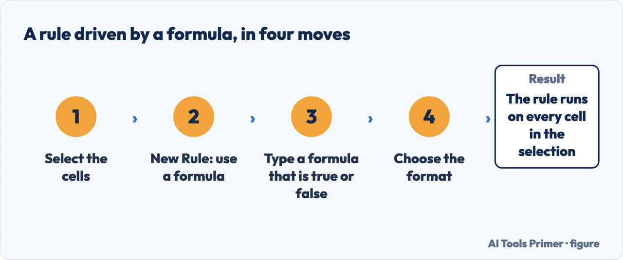
Drawn flow of the four steps to a conditional formatting rule driven by a formula in Excel — Four moves, and the rule then runs once per cell in the selection. Figure drawn by AI Tools Primer.

Select the cells the rule should run on. Select them before you open the dialog: the selection becomes the rule’s Applies to range, and it is also what every reference in your formula will be measured against.
Home › Conditional Formatting › New Rule. Then, under Select a Rule Type, choose Use a formula to determine which cells to format.
Type a formula that is either true or false for one cell. Start with an equals sign. Write it for the top-left cell of the selection — =$F5="TX", not a formula that tries to describe the whole range at once.
Decide which part of the reference is locked before you leave the box. A dollar sign freezes what follows it. $F5 means always column F, whichever row this cell is on, and that is what makes a rule colour whole rows.
Click Format, choose the fill, font or border, and save. You can pick more than one kind of formatting, and Excel shows the combination in the Preview box before you commit.

Why the presets run out

Excel ships with rules you can pick from a list. A formula is what you use when the list does not have the condition you need.

A preset

Greater than, between, duplicate values, top ten, colour scales. Quick, and each one tests the cell it is colouring. If the condition is about that cell’s own value, a preset is the right tool and a formula adds nothing.

A formula

Anything else. Microsoft’s own reason for it: you may want to “compare values in a selection to a result returned by a function or evaluate data in cells outside the selected range”. That is the whole difference — the condition can look somewhere other than the cell being coloured.

Drawn table of three ways to write the same conditional formatting reference in Excel and what each one colours — The dollar signs are the rule. Figure drawn by AI Tools Primer from Microsoft and Exceljet, both read on 24 September 2026.

The sentence that decides whether your rule works

Microsoft prints this twice on the same page, each time in a Note: “Selecting cells on the worksheet inserts absolute cell references. If you want Excel to adjust the references for each cell in the selected range, use relative cell references.”

In plain terms: if you built the formula by clicking a cell, Excel wrote $F$5 — frozen in both directions. That single reference is then tested for every cell in the selection, so either all of them go red or none of them do. It looks like the rule is broken. It is doing exactly what it was told.

Exceljet gives the mental model that makes this stop being confusing: imagine typing the formula into the top-left cell of the selection and then copying it across the whole range, with references updating as usual. Whatever that copy would do to the reference is what the rule does.

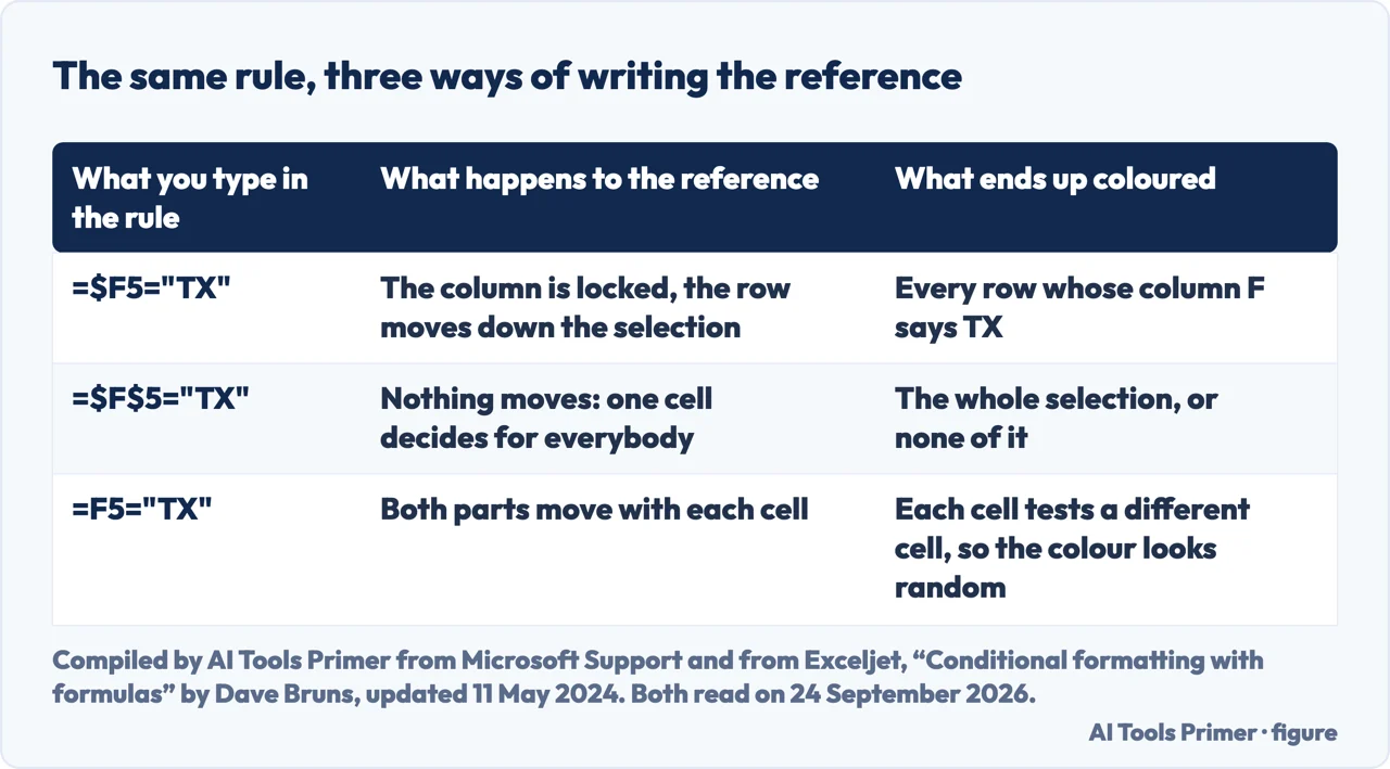
The clearest way to see this is a rule that colours whole rows. Select the table, and use a formula that locks the column and leaves the row free — =$F5="TX" in Exceljet’s worked example. Because the column is frozen, every cell in a given row asks the same question: what does column F say on my row. Because the row is not frozen, the question changes as the rule works down the table. Lock both parts and the whole selection asks about row 5. Lock neither and each cell asks about a different cell entirely, and the colouring looks random.

Drawn table of three reasons an Excel conditional formatting rule does not fire, with the sign each one leaves — Each cause leaves a different sign, which is what makes them worth checking in this order. Figure drawn by AI Tools Primer.

When a correct-looking rule does nothing

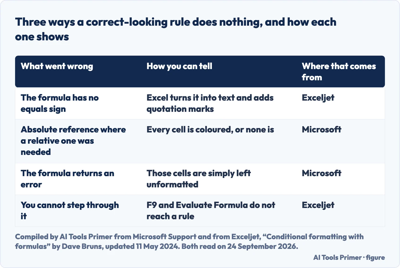
Three causes, in the order worth checking them. Each one leaves a different sign.

The equals sign is missing: Check this first because it is silent and instant. Exceljet: “If you forget this step, Excel will silently convert your entire formula to text, rendering it useless.” The sign is that quotation marks have appeared around your formula in the rule. Remove them, put the equals sign back.
The reference is locked when it should move: The sign is that every cell is coloured, or none is. Open Manage Rules, look at the formula, and take the dollar signs off whichever part needs to follow the cell — usually the row number.
The formula returns an error: Microsoft: “If any cells contain a formula that returns an error, conditional formatting is not applied to those cells.” The sign is a rule that works everywhere except a few cells. Their suggested fix is to wrap the condition in an IS function or IFERROR so it returns something you chose instead of an error.
And the thing that makes all three harder to find: You cannot step through a conditional formatting formula. F9 and Evaluate Formula, the two tools for examining any other formula in Excel, do not reach inside a rule. Exceljet’s way round it is a dummy formula: type the same formula into a block of empty cells shaped like your data and read the TRUEs and FALSEs off the sheet.

There are three things a formula rule cannot do, and they are worth knowing before you spend an afternoon on one that was never going to work.

No icons, bars or colour scalesA formula rule can set number format, font, fill and borders. The graphical styles are not available to a formula rule.

No unions, intersections or array constantsSome of these can be worked round by moving the logic into a cell and pointing the rule at that cell instead.

No references to another workbookAnother sheet in the same workbook is fine. Another file is not.

What happens when a rule and ordinary formatting disagree. Microsoft is explicit: if a rule evaluates as true, “it takes precedence over any existing manual format for the same selection”, and “if you delete the conditional formatting rule, the manual formatting for the range of cells remains”. So a cell you coloured by hand keeps that colour underneath, invisible, until the rule stops being true or is removed. Manual formatting is also not listed in the Rules Manager, so a colour that nothing in the list explains may not be conditional at all.

A formula rule is also the documented way round a limit of the duplicate-values preset. Microsoft notes that with authoring languages that use double-byte characters, such as Japanese, halfwidth and fullwidth characters are treated as the same value; if you need to tell them apart, the answer is a rule built on COUNTIF instead. It is a narrow case, and it has the shape of many reasons to write a formula: the preset is right about nearly everything and wrong about the one thing that matters to you. The same reasoning applies to removing duplicates, where seeing them before deleting anything is usually the safer order.

One habit saves most of the trouble. Build the formula by typing the references rather than by clicking cells. Clicking is what inserts the absolute reference that breaks the rule. If you do click, look at the formula before you press OK and take off the dollar signs you did not mean. The same care over what an operator actually means applies to the not-equal comparison, which is written differently in a formula and in a criteria box.

The rule type, the two requirements, the note about absolute and relative references, the precedence over manual formatting and the error behaviour are quoted from Microsoft’s Excel documentation. The four-step summary, the copy-across mental model, the silent conversion to text and the dummy-formula technique are from Exceljet. Both were read on 24 September 2026 and are listed below; the order of the three causes, and the advice to type references rather than click them, are ours.

Where to start

Four ways in.

“The list of rules does not have what I need.”: That is what a formula is for — why the presets run out
“I want the four steps.”: Start at writing the rule
“It colours the wrong cells.”: The dollar signs — what the reference decides
“Nothing happens at all.”: Three causes — when nothing fires

Why the presets run out

A preset tests the cell it colours. A formula can look anywhere else, and that is the only real difference.

Removing duplicates in ExcelThree tools and only one deletes, and what Excel actually counts as a duplicate.Open this guide → Does not equal in ExcelTwo characters, and the four places where they are written differently.Open this guide → Comparing two Excel filesMicrosoft’s tool is restricted to enterprise Windows — and one helper column does the job anywhere.Open this guide →

Writing the rule

Five steps, and the one of them that people skip is choosing what the selection is before the dialog opens.

Wrapping text in ExcelTwo different ways, which one suits which kind of content, and the two documented reasons the wrapped text stays invisible.Open this guide → Freezing rows in ExcelOne rule from Microsoft explains every case, including the two that send people to forums.Open this guide → Percentages in ExcelThe formulas are the easy half. The format changes the number, and does something different depending on when you apply it.Open this guide →

What the reference decides

Absolute or relative, written by a dollar sign, and it is the difference between colouring a table and colouring one cell.

VLOOKUPFour arguments, and the optional one that returns wrong answers without reporting anything.Open this guide → XLOOKUPThe six arguments, and the four cases where it beats the older lookup.Open this guide → Locking cells in ExcelEvery cell is already locked, so the real job is unlocking the ones people should edit.Open this guide →

When nothing fires

The equals sign, the locked reference and the error, in that order. Each leaves its own sign.

Enabling macros in ExcelThe yellow bar, the four settings, and the internet block with no button at all.Open this guide → Alphabetising in ExcelOne word in Microsoft’s first step keeps your rows together, and two documented failures explain every list that sorts wrong.Open this guide → Merging cells in ExcelMicrosoft says merging deletes the other cells — and there is a different command for what was meant.Open this guide →

Questions people also ask

How do I create a formula in Excel to change colour based on a value?

Select the cells, then Home › Conditional Formatting › New Rule › Use a formula to determine which cells to format. Enter a formula that starts with = and returns TRUE or FALSE for the top-left cell of the selection, then click Format and choose the fill or font colour.

Why does my conditional formatting colour the wrong cells?

Check the dollar signs first. Microsoft warns that clicking cells to build the formula inserts absolute references, so the same cell is tested for the whole selection. Remove the dollar sign from whichever part should change as the rule moves — usually the row number.

Why is my conditional formatting formula not working at all?

Check the equals sign first. Without it Excel stores the rule as text and wraps it in quotation marks, and nothing fires. If the formula is right, the next candidates are a locked reference and cells whose formulas return an error, which Excel leaves unformatted.

Can I use conditional formatting based on another cell?

Yes — that is what a formula rule is for. Microsoft describes the case as evaluating “data in cells outside the selected range, which can be in another worksheet in the same workbook”. Another workbook is not allowed.

Can I apply data bars or icons with a formula?

No. Exceljet lists this as the first limit: a formula rule can set number format, font, fill colour and borders, not icons, colour scales or data bars.

Not covered here. It does not cover the preset rules one by one. They are the right tool whenever the condition is about the cell being coloured, and they need no explaining.

It does not cover Google Sheets.

And it does not recommend an add-in. Everything here is in the dialog Excel already has. What holds instead is simple: the rule type and the note about references are quoted from Microsoft’s own Excel documentation, with the date it was read.

Sources

Microsoft Support — Use conditional formatting to highlight information in Excel: the formula rule type, the equals-sign and TRUE requirements, the note about absolute and relative references, precedence over manual formatting and the error behaviour. Applies to Windows editions; no Mac edition is listed — support.microsoft.com, read September 2026.
Exceljet — Conditional formatting with formulas, by Dave Bruns, updated 11 May 2024: the four-step summary, the copy-across model, the silent conversion to text, the dummy-formula technique and the three limitations — exceljet.net, read September 2026.

Written by Alberto Gulotta

Founder and editor of AI Tools Primer, writing from Palermo, Italy. Thirty-five years of taking computers apart, starting with a Commodore 64 — the long version is on the about page.

Something wrong on this page? Write to aitoolsprimer@gmail.com and it gets fixed.

Written on 24 September 2026.

Independence and limits

No affiliate links and no paid placements anywhere on this site. Nobody pays to appear here, and no company has seen this page before you did.

This is general information, not professional advice. Where a page touches money, health, safety or the law, it names its source and the date it was read — and your situation may still differ. See the privacy page and the cookie policy.