
Docs · guide
How to use vlookup in excel, and the argument to always type
By Alberto Gulotta · Updated · 9 min read
The mechanics of how to use vlookup in excel are four arguments long and Microsoft documents them precisely. Three of them are straightforward. The fourth is optional, and leaving it out is how a spreadsheet returns confident wrong answers for months.
The plain-language version Microsoft gives is a good place to start: VLOOKUP says “what you want to look up, where you want to look for it, the column number in the range containing the value to return, return an Approximate or Exact match”.
The four arguments, and which of them bites
- lookup_value
- What you are looking for. Microsoft’s constraint: it “must be in the first column of the range of cells you specify in the table_array argument”. If table_array is B2:D7, the thing you are looking up has to be in column B.
- table_array
- The range to search. Its first column must hold the lookup value, and the range must also contain the answer you want back.
- col_index_num
- Which column returns the answer — “starting with 1 for the left-most column of table_array”. Counted inside the range, not across the sheet. This is why inserting a column breaks a working formula.
- [range_lookup]
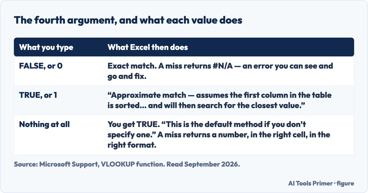
- Optional, and the most dangerous optional argument in Excel. 0/FALSE means exact match. 1/TRUE means approximate — and it is what you get when you leave the argument out.
Before the fourth argument, the structural rule that causes the other half of the failures. Microsoft states it as a tip and it is really a constraint: “the secret to VLOOKUP is to organize your data so that the value you look up (fruit) is to the left of the return value (amount) you want to find.” VLOOKUP only looks rightwards from its first column. If the thing you know is to the right of the thing you want, no amount of adjusting the formula will help — the columns have to move, or the function has to change.
Now the argument that matters most.
“Approximate match — 1/TRUE assumes the first column in the table is sorted either numerically or alphabetically, and will then search for the closest value. This is the default method if you don’t specify one.”
Microsoft, on the fourth argument. Read the two halves together, because between them they explain most of the wrong answers spreadsheets have ever produced. The default assumes your data is sorted, and if it is not, it does not stop — it returns the closest value it found on the way.
The two failure modes are not equally visible. An exact-match miss returns #N/A, which is an error you can see and go and fix. An approximate-match miss returns a number, in the right format, in the right cell, that is simply the wrong number. Nothing is highlighted. Nothing is reported. It goes into the total.
Which gives the single most useful habit in this entire subject: type the fourth argument every
time. Almost always FALSE. Leaving it off is not shorter, it is a different
function.
It is worth being concrete about how this goes wrong in practice, because it does not look like an error at any point. A lookup of employee IDs against an unsorted list, with the fourth argument omitted, will return a name for every row. Some of those names belong to the wrong employee. The sheet totals correctly, prints correctly, and is wrong. The people who find these usually find them a quarter later, when a number does not reconcile.
The second most common failure is the one the third argument causes, and it has the same character: it appears after the formula was working. col_index_num is a count inside the range, so a formula returning column 3 of A:E keeps pointing at the third column even after somebody inserts a new column at B — and the third column is now something else entirely. Named ranges and tables reduce this, and Microsoft notes you can use them instead of cell references.
And before any of this, the sentence Microsoft puts at the very top of its own VLOOKUP page: “Try using the new XLOOKUP function, an improved version of VLOOKUP that works in any direction and returns exact matches by default, making it easier and more convenient to use than its predecessor.”
That is the vendor recommending you not use the thing you came to read about. Both of the traps on this guide — the left-hand column rule and the dangerous default — are ones XLOOKUP removes by design. If your Excel has it, the honest answer to “how do I use VLOOKUP” is often “use the other one”. VLOOKUP still matters because it is in millions of existing spreadsheets, and reading those is a different job from writing new ones.
A practical note on looking things up across sheets, since Microsoft gives the form: =VLOOKUP(A2,'Client Details'!A:F,3,FALSE). Whole-column references like A:F work and are convenient; on very large workbooks they are also more work than a defined range, which is the trade to be aware of rather than a rule.
On the phrasing: how to use vlookup without naming the program is very nearly the same question, because Google Sheets has the function with the same shape — VLOOKUP(search_key, range, index, is_sorted) — and the same trap. Google’s own documentation is blunter than Microsoft’s about it: FALSE is “for an exact match, this is recommended”, while TRUE “is the default if is_sorted is unspecified”. Two companies, the same optional argument, the same advice to always supply it.
And if the answer comes back as #N/A, that is the honest failure rather than the dangerous one. It means the value was genuinely not found in the first column of the range — usually because of a stray space, a number stored as text, or a lookup value that is not in the first column at all. All three are checkable in a minute, and none of them are the formula being broken.
The guides below take it four ways: the function itself, the errors it produces, what to use instead, and the spreadsheet habits that make lookups reliable in the first place.
Where to start
Four ways in.
- “I need to write one now.”
- Start at the function
- “My data is the wrong way round.”
- That is what to use instead
- “It worked and now it does not.”
- That is keeping it reliable
The function
Four arguments, one of them optional and dangerous. These guides take each in turn, in the order they cause trouble.
What to use instead
Microsoft’s own first recommendation on its VLOOKUP page is a different function. This wing takes that seriously.
Keeping it reliable
Most lookup failures are data failures wearing a formula costume. These guides are about the sheet underneath.
Not covered here. It will not tell you to leave the fourth argument off. Microsoft documents what happens when you do, and it is the quietest way to be wrong in a spreadsheet.
It will not pretend VLOOKUP is the modern answer. Microsoft recommends XLOOKUP at the top of its own VLOOKUP page, and repeating that is more useful than defending the old function.
And it will not give you a formula to paste without the ranges. The ranges are the whole of it, and they are specific to your sheet. What holds instead is simple: the constraint on the first column and the recommendation to use XLOOKUP are Microsoft’s own, quoted from its VLOOKUP page.
Step 4 of 21 in half an hour in a spreadsheet
The order the work actually happens in: the data arrives, it gets cleaned, it gets counted, it gets a chart, and then somebody else opens it.
- Before this
- How to alphabetize in Excel, without scrambling your rows
- After this
- How to calculate percentage in Excel, and the format trap
Getting an answer out of a spreadsheet
Four jobs that all end with a number somebody asked you for.
- The same job, in the other places it comes up
- How to create a pivot table in excel, starting with the data
- How to remove duplicates in Excel, and what counts as one
- How to compare two Excel files, with or without the tool
Sources
- Microsoft Support — VLOOKUP function (the syntax and all four arguments, the requirement that the lookup value sit in the first column, col_index_num counted inside the range, the statement that approximate match assumes sorted data and is the default, and the recommendation to try XLOOKUP instead) — support.microsoft.com, read 6 September 2026.
- Google Docs Editors Help — VLOOKUP (the same four arguments in Google Sheets, that is_sorted is optional, that FALSE is recommended for an exact match, and that TRUE is the default when it is left unspecified) — support.google.com, read 22 August 2026.
Written by Alberto Gulotta
Founder and editor of AI Tools Primer, writing from Palermo, Italy. Thirty-five years of taking computers apart, starting with a Commodore 64 — the long version is on the about page.
Something wrong on this page? Write to aitoolsprimer@gmail.com and it gets fixed.
Written on 22 August 2026 · last checked 23 September 2026.
Independence and limits
No affiliate links and no paid placements anywhere on this site. Nobody pays to appear here, and no company has seen this page before you did.
This is general information, not professional advice. Where a page touches money, health, safety or the law, it names its source and the date it was read — and your situation may still differ. See the privacy page and the cookie policy.