
Docs · guide
Does not equal in Excel: two characters, four different spellings
By Alberto Gulotta · Updated · 11 min read
The does not equal in excel operator is <> — less-than then greater-than, no space. That is the whole answer for a formula. It stops being the whole answer the moment you put it inside COUNTIF or SUMIF, where it has to be written as text and joined to its value with an ampersand, and where getting that wrong produces a number rather than an error.
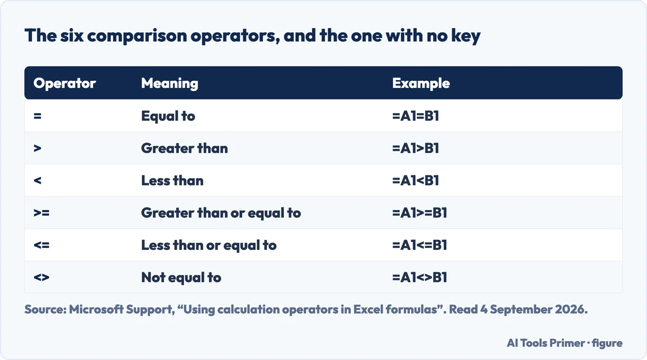
| Operator | Meaning | Example |
|---|---|---|
= | Equal to | =A1=B1 |
> | Greater than | =A1>B1 |
< | Less than | =A1<B1 |
>= | Greater than or equal to | =A1>=B1 |
<= | Less than or equal to | =A1<=B1 |
<> | Not equal to | =A1<>B1 |
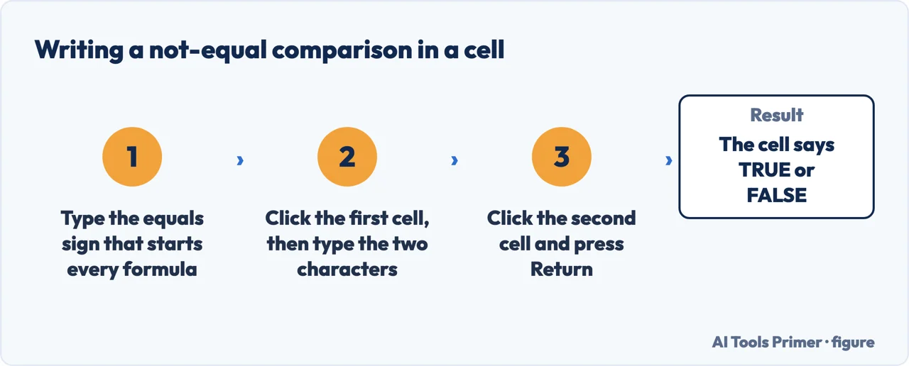
- Click an empty cell and type an equals sign. Every formula starts there, including a
comparison — the first
=means “calculate this”, not “equals”. - Type the first value or click its cell. Clicking is safer than typing a reference, because Excel writes it correctly and colours it on the sheet.
- Type the two characters
<>. Less-than then greater-than, no space between them. There is no key for “not equal” on the keyboard and no other spelling Excel accepts. - Type the second value or click its cell, then press Return. The cell now says TRUE or FALSE. Microsoft’s rule for the whole family: “when two values are compared by using these operators, the result is a logical value — either TRUE or FALSE”.
- Wrap it in IF if you want words instead.
=IF(A1<>B1,"changed","same")turns the logical value into something a reader can act on. - If you are counting rather than comparing, stop here. Inside COUNTIF and SUMIF the same two characters have to be written differently, and that is the next section.
The same operator, in the four places people use it
Only the first one is written the way you would expect. The other three put
<> inside quotation marks, and that is where the wrong answers come from.
=A1<>B1
=IF(A1<>B1,"changed","same")
=COUNTIF(B2:B5,"<>75")
=COUNTIF(B2:B5,"<>"&B4)
Why <>A1 inside COUNTIF gives the wrong number and no error
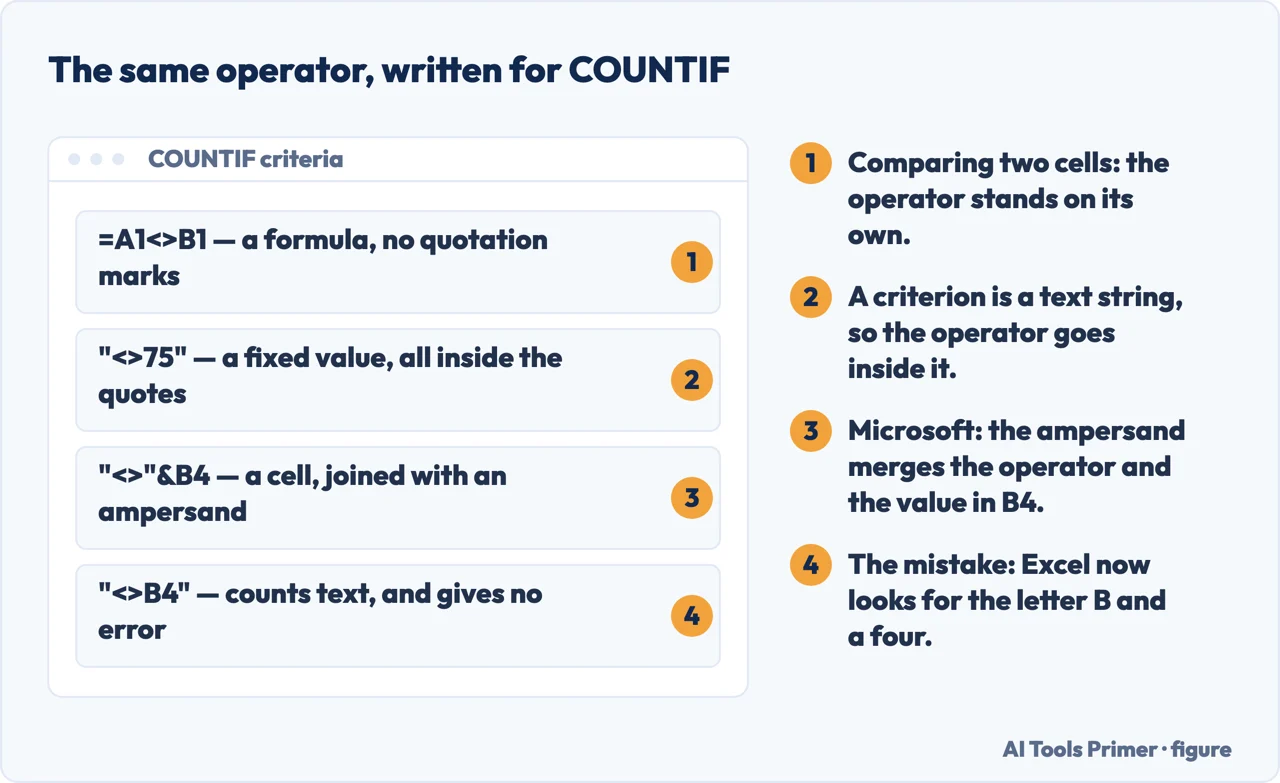
Because COUNTIF does not take a comparison. It takes a criterion, and a criterion is a piece
of text. Microsoft defines the argument as “a number, expression, cell reference, or text
string that determines which cells COUNTIF counts”, and gives ">32" as the
example of a comparison written as one. The quotation marks are not decoration: they are what turns
an operator into something COUNTIF can read.
So the value has to be glued on, not typed in. Microsoft’s worked line is exact:
=COUNTIF(B2:B5,"<>"&B4) “counts the number of cells with a value not
equal to 75”, and the explanation is that “the ampersand (&) merges the comparison
operator for not equal to ("<>") and the value in B4 to read
=COUNTIF(B2:B5,"<>75")”. Write "<>B4" instead and Excel
counts the cells that do not contain the letter B followed by a four.
Nothing about that is flagged. You get a whole number, in the right cell, of a plausible size. It is the same class of fault as an approximate lookup: an answer, not an error. If a count seems too high by roughly the number of rows in the range, the missing ampersand is the first thing to check.
“Not equal to nothing”, and the cell that only looks empty
<>"" is how people write “this cell has something in it”, and most
of the time it is right. The exception is worth knowing because it is invisible: a cell holding a
formula that returns an empty string — something like
=IF(A1>10,"high","") — is not blank. It contains a formula, and its result is
a text value that happens to have no characters.
So two reasonable-looking tests disagree. =A1<>"" says the cell is empty,
because the value is an empty string. ISBLANK says it is not, because there is a formula in it.
Neither is broken; they are answering different questions, one about the value and one about the
cell. On a column of formulas, that difference decides whether a count is right.
The practical version. Use <>"" when you care about what is displayed,
and ISBLANK when you care about whether anything was ever put there. And if a row count disagrees
with what you can see on screen, a column of formulas returning "" is the usual
reason.
Text comparisons ignore capitals, and that surprises people twice. =A1<>B1 on the words “Apples” and “apples” returns FALSE: to Excel they are the same value. Microsoft says the same of the counting functions — criteria “aren’t case sensitive”, so “the string "apples" and the string "APPLES" match the same cells”. If capitals genuinely matter, the comparison to reach for is EXACT, which is the only one that sees them.
The other reason two identical-looking cells are not equal. A trailing space. “Smith” and “Smith ” are different values and look identical in every font ever made. Microsoft’s own advice on counting is to “make sure your data doesn’t contain erroneous characters” — leading spaces, trailing spaces, straight against curly quotation marks. When a comparison insists two things differ and you can see they do not, TRIM on a spare column settles it in a second.
A number that is really text is the third case. Data pasted from a web page or a PDF often arrives as text, and text 75 is not equal to number 75. The tell is the alignment: Excel puts numbers on the right of a cell and text on the left by default, so a column that is ragged down the left edge is a column of numbers, and one aligned left is a column of text pretending.
Where the operator changes meaning entirely. Advanced Filter, conditional formatting rules and data validation all accept criteria, and each has its own idea of whether the operator wants quotation marks. The rule that survives all of them: if the box you are typing into expects a criterion rather than a formula, the operator is text; if it expects a formula, it is not.
The same rule, in the other program. Google’s own documentation for Sheets writes the criterion the same way — COUNTIF(A1:A10,">20") — and defines the argument as “the pattern or test to apply”. So a formula that counts correctly in Excel usually counts correctly in Sheets, and one that forgot the quotation marks is wrong in both. That is worth knowing before a workbook is converted rather than after.
The operator table, the criteria definition and the worked COUNTIF line are quoted from Microsoft’s own Excel documentation and from Google’s Sheets documentation, read on 4 September 2026 and listed below. The note on empty strings, trailing spaces and text numbers is ours.
Where to start
Four ways in.
- “I just need the symbol.”
- It is
<>— then the four places - “My COUNTIF is wrong.”
- Quotation marks and ampersand — the countif trap
- “Two identical cells say not equal.”
- Spaces or text numbers — see when equal things are not
- “I want words, not TRUE.”
- Wrap it in IF, step five the four places
The four places
One operator, written two different ways depending on whether Excel is expecting a formula or a criterion. Everything else follows from that distinction.
The COUNTIF trap
A criterion is a piece of text, so the operator goes inside the quotation marks and the value is joined on. Get it wrong and you get a number, not an error.
When equal things are not
Trailing spaces, capital letters and numbers stored as text: three reasons a comparison disagrees with your eyes, and none of them shows on screen.
Where the result goes
TRUE and FALSE are rarely the destination. They feed an IF, a count, a colour rule or a chart, and each one reads them slightly differently.
Questions people also ask
What is the does not equal sign in Excel?
Two characters typed together: <>. Microsoft lists it among the comparison operators as “not equal to”, with =A1<>B1 as the example.
How do I write not equal in an IF statement?
The same way, with no quotation marks around the operator: =IF(A1<>B1,"changed","same"). The comparison sits inside the first argument of IF exactly as it would on its own.
Why does my COUNTIF with <> give the wrong count?
Because inside COUNTIF the condition is a text string. Use "<>75" for a fixed value, and "<>"&B4 for a cell — the ampersand “merges the comparison operator for not equal to” with the value.
Is there a NOT function I should use instead?
There is, and it does the same job the long way round: =NOT(A1=B1) equals =A1<>B1. NOT earns its place when it wraps something more complicated than a single comparison.
How do I count cells that are not empty?
=COUNTIF(range,"<>") counts cells with anything in them. Be aware that a formula returning an empty string counts as having something, which is why it can disagree with what you see on screen.
Not covered here. It will not list every function that accepts a criterion. The rule — criterion means text, formula means no quotation marks — covers the ones it does not name.
It will not teach the IF function properly, which is a bigger subject and deserves its own page.
And it will not tell you a comparison is broken when the data is. Spaces and text numbers are a data problem wearing a formula’s clothes. What holds instead is simple: the operator table, the criteria definition and the worked COUNTIF example are quoted from Microsoft’s own Excel documentation, with the date each page was read.
Sources
- Microsoft Support — Using calculation operators in Excel formulas: the comparison operator table, including <> for not equal to, and the rule that the result is TRUE or FALSE — support.microsoft.com, read 4 September 2026.
- Microsoft Support — Use the COUNTIF function in Microsoft Excel: the definition of a criterion as a text string, the case-insensitivity note, and the worked example =COUNTIF(B2:B5,"<>"&B4) — support.microsoft.com, read 6 September 2026.
- Google Docs Editors Help — COUNTIF in Google Sheets: the same criterion-as-text rule in the other spreadsheet, read as a check that the behaviour is not a Microsoft peculiarity — support.google.com, read 4 September 2026.
Written by Alberto Gulotta
Founder and editor of AI Tools Primer, writing from Palermo, Italy. Thirty-five years of taking computers apart, starting with a Commodore 64 — the long version is on the about page.
Something wrong on this page? Write to aitoolsprimer@gmail.com and it gets fixed.
Written on 4 September 2026 · last checked 7 September 2026.
Independence and limits
No affiliate links and no paid placements anywhere on this site. Nobody pays to appear here, and no company has seen this page before you did.
This is general information, not professional advice. Where a page touches money, health, safety or the law, it names its source and the date it was read — and your situation may still differ. See the privacy page and the cookie policy.