Docs · guide

How to unhide columns in Excel, including column A

By Alberto Gulotta · Updated 23 September 2026 · 12 min read

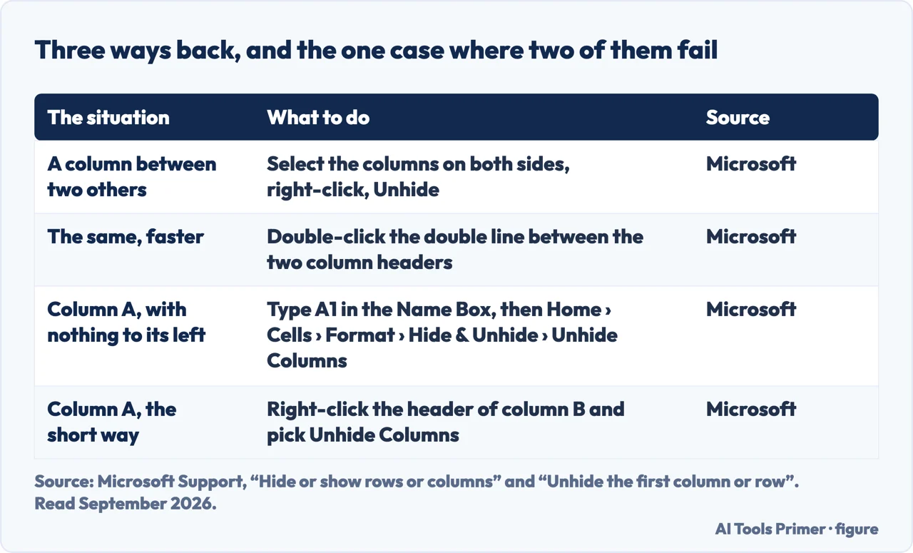
How to unhide columns in Excel: select the columns on both sides of the gap, right-click, Unhide. That works for every column except one. Column A has a Microsoft support page of its own, and the reason is a single sentence of geometry.

Four ways back, and the one situation where two of them do not work
The situation	What to do	Why it works	Source
A column between two visible ones	Select the columns on both sides, right-click, Unhide	You can select round the gap	Microsoft
The same, without the menu	“Double-click the double line between the two columns where hidden columns exist”	The double line is the indicator that something is hidden	Microsoft
Column A	Right-click the header of column B and pick Unhide Columns	There is nothing to the left to select	Microsoft
Column A, when that fails	Type `A1` in the Name Box, then Home › Cells › Format › Hide & Unhide › Unhide Columns	The Name Box selects a cell you cannot click	Microsoft
The same in Google Sheets	“Click the arrow where the row number or column letter used to be”	Sheets marks the gap with an arrow instead of a double line	Google

Table of four ways to unhide columns in Excel, including the special case of column A — Three of the four need something to the left of the gap. Figure drawn by AI Tools Primer.

The ordinary case, and how to see it coming

Everything here is from Microsoft’s page on hiding and showing.

The tell: “The double line between two columns is an indicator that you’ve hidden a column.” On a wide sheet this is easier to miss than with rows, because column letters skipping from C to F is a small change to notice.
The method: “Select the adjacent columns for the hidden columns”, right-click them, then Unhide.
The shortcut: “Or, double-click the double line between the two columns where hidden columns exist.” Fastest when you can see exactly where the gap is.
All at once: Select the whole worksheet, then Home › Cells › Format › Hide & Unhide › Unhide Columns. Microsoft’s caveat applies: this “displays all hidden rows and columns … which you may not want to do”.

And the reason the command sometimes is not there at all: “If you don’t see Unhide Columns or Unhide Rows, make sure you’re right-clicking inside the column or row label” — the lettered strip along the top, not the cells beneath it.

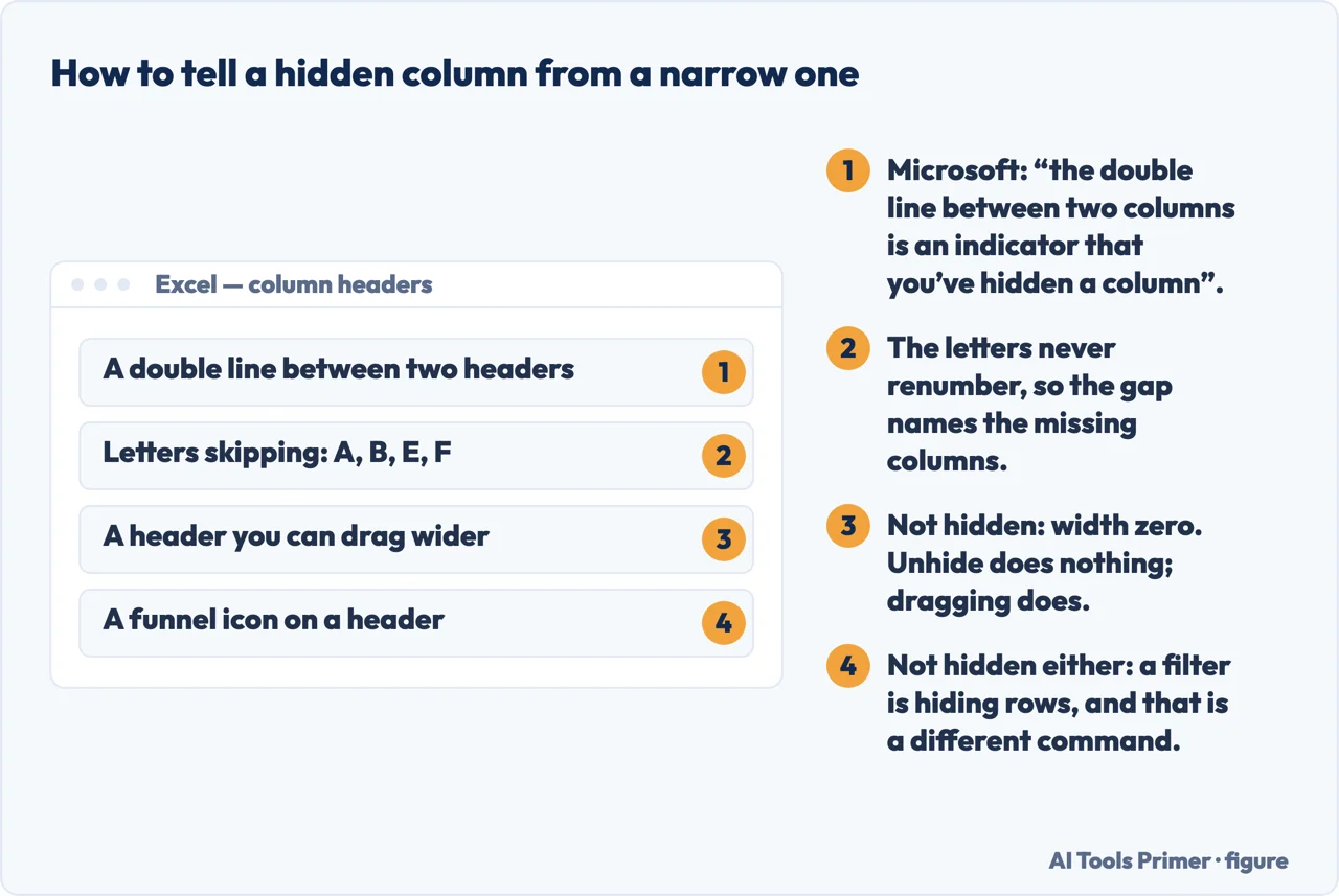
Look at the column letters. They never renumber, so a jump from B to E names exactly what is missing. A double line between two headers is Microsoft’s own indicator “that you’ve hidden a column”.
Select the columns on both sides of the gap. Click the header on the left, then shift-click the one on the right.
Right-click the selection and choose Unhide. Or double-click the double line between the two headers, which does the same thing without a menu.
For column A, right-click the header of column B and pick Unhide Columns. There is nothing to its left to select, which is the whole reason this case has its own page at Microsoft.
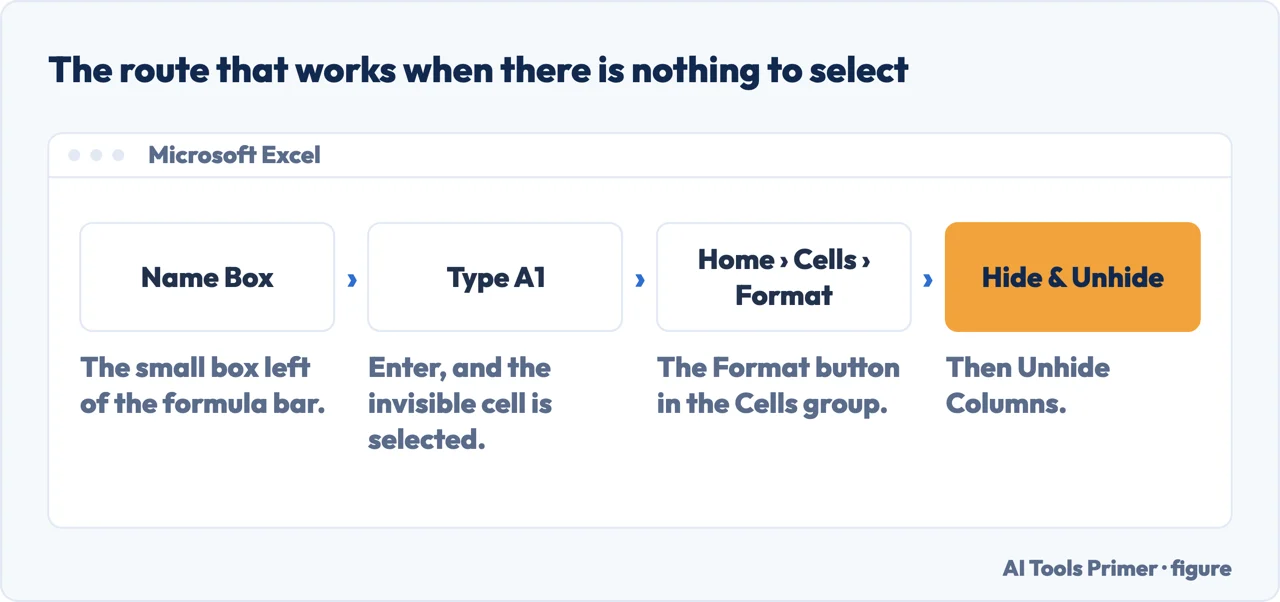
If that does not work, select the invisible cell by name. Type A1 in the Name Box next to the formula bar, press Enter, then Home › Cells › Format › Hide & Unhide › Unhide Columns.

“If the first row (row 1) or column (column A) is not displayed in the worksheet, it is a little tricky to unhide it because there is no easy way to select that row or column.”

Microsoft, read 22 August 2026. Column A is a searched-for problem in its own right, and this is why: the usual method needs the columns on both sides, and column A only has one. There is nothing to the left of it to include in the selection.

Two ways in, both from the same page. The Name Box, beside the formula bar: type A1 and press Enter. Or Home › Editing › Find & Select › Go To, with A1 in the Reference box. Either one puts the cursor in a cell you cannot click on.

Then Home › Cells › Format › Hide & Unhide › Unhide Columns. There is also a simpler route Microsoft gives for the web version: “right-click the column B header or label and pick Unhide Columns”.

The Name Box route to select cell A1 and unhide the first column in Excel — The Name Box reaches a cell the mouse cannot. Figure drawn by AI Tools Primer.

One thing that cannot be the cause, and it saves you time

When rows go missing, a filter is one of the likeliest explanations — Microsoft describes filtered data as showing “only the rows that meet criteria that you specify” and hiding the rest. Note the word: rows.

A filter does not remove columns. So if letters are missing from the top of your sheet, filtering is not what happened, and you can stop looking for a funnel icon. It is one of four things: the columns are hidden, one of them is column A, the width has been set to almost nothing, or you are right-clicking in the wrong strip.

That last possibility for width is worth checking before you conclude anything, and it uses the same menu: Format › Cell Size › Column Width, then type a value. A column at a width of zero looks exactly like a hidden one and will not respond to Unhide.

How to tell a hidden Excel column from one that is only zero-width or filtered — Two of these four are not hidden at all, and Unhide will not touch them. Figure drawn by AI Tools Primer.

The same gap looks different in Google Sheets. There is no double line: Google marks a hidden row or column with an arrow, and its instruction for getting it back is “click the arrow where the row number or column letter used to be”. A file that moves between the two programs keeps the hidden columns and changes the sign that tells you they are there.

Why this is worth two minutes rather than one click. A spreadsheet that arrives with columns missing usually arrived that way on purpose: somebody hid the working columns before sending it, or hid a column of costs before showing the sheet in a meeting. Unhiding everything is the fastest way to see the data and also the fastest way to put something on screen that was deliberately taken off it. If the file came from someone else, unhide the specific gap rather than the whole sheet.

And the reverse, if you are the sender. Hidden columns are not removed — they are in the file, and one right-click away for anybody who receives it. Hiding is a tidying device, not a redaction. If a column genuinely must not travel, the answer is to delete it from a copy of the workbook, and to check afterwards that no formula elsewhere still refers to it.

One small habit that prevents the confusion entirely. When you hide working columns in a sheet other people will open, put a note in a cell at the top saying which letters are hidden and why. It takes a line, it survives being emailed, and it turns a puzzle into a piece of information.

The methods, the double line indicator, the note about column A, the Name Box and Go To routes, the right-click tip and the description of what a filter hides are quoted from Microsoft’s own Excel documentation, read on 22 August 2026 and listed below. The point that a filter cannot explain missing columns, and the advice about hiding as tidying rather than redaction, are ours.

Where to start

Four ways in.

“The letters skip from C to F.”: Ordinary case — the ordinary case
“Column A is gone.”: It needs a different route — column a
“Unhide is not in the menu.”: Check where you are right-clicking — the ordinary case
“Could it be a filter?”: No, and that saves you time — what it cannot be

The ordinary case

Select either side and right-click, or double-click the double line. Both are Microsoft’s, and one of them is much faster.

Hidden rows in ExcelThree clicks — and the four reasons they fail, including the one where the rows were never hidden.Open this guide → Does not equal in ExcelTwo characters, and the four places where they are written differently.Open this guide → Freezing rows in ExcelOne rule from Microsoft explains every case.Open this guide → Wrapping text in ExcelTwo different ways, which one suits which kind of content, and the two documented reasons the wrapped text stays invisible.Open this guide →

Column A

It has no neighbour on the left, so the usual method has nothing to grip. Microsoft gives it its own page.

Sorting alphabeticallyOne word in Microsoft’s first step keeps your rows together.Open this guide → Merging cells in ExcelMicrosoft says merging deletes the other cells, and merged blocks break everything downstream.Open this guide → Lock cells in ExcelEvery cell is already locked, so the real job is unlocking the ones people should edit.Open this guide →

What it cannot be

Filters hide rows, not columns. Ruling that out immediately leaves four possibilities instead of five.

Comparing two workbooksMicrosoft’s tool is restricted to enterprise Windows — and one helper column does the job anywhere.Open this guide → Removing duplicates in ExcelThree tools and only one deletes, and what Excel actually counts as a duplicate.Open this guide → PDF to ExcelWhat survives the conversion, and the numbers that arrive as text.Open this guide →

Before you send it on

A hidden column is still in the file. Hiding tidies a sheet; it does not remove anything from it.

Checkboxes in ExcelHere the box is the cell’s value, so the ticks can be counted.Open this guide → Drop-down lists in ExcelPut the source in a table so it updates itself, and the option that decides whether the list is enforced.Open this guide →

Questions people also ask

How do I unhide columns in Excel?

Select the columns on either side of the gap, right-click, and choose Unhide. Faster still: double-click the double line between the two headers — Microsoft names that line as the indicator that a column is hidden.

How do I unhide column A?

Right-click the header of column B and pick Unhide Columns. If that does not reach it, type A1 in the Name Box next to the formula bar, press Enter, then use Home › Cells › Format › Hide & Unhide › Unhide Columns.

How do I unhide all the columns at once?

Select the whole worksheet, then Home › Cells › Format › Hide & Unhide. Microsoft warns what that costs: it “displays all hidden rows and columns in your worksheet, which you may not want to do”, and a sheet often hides columns for a reason.

Why does Unhide do nothing?

Because the column may not be hidden. A column set to zero width looks the same and is fixed by dragging or by setting a Column Width; and rows that vanish under a filter are a different command again. Unhide only reverses Hide.

Not covered here. It will not give one method for every column. Column A has no left-hand neighbour, and Microsoft gives it a page of its own for that reason.

It will not send you looking for a filter. Filters hide rows, so a missing column is never that.

And it will not describe hiding as a way of removing something. A hidden column is in the file, one right-click away. What holds instead is simple: the note about column A and the description of what a filter hides are Microsoft’s own, quoted with the date each page was read.

Step 16 of 21 in half an hour in a spreadsheet

The order the work actually happens in: the data arrives, it gets cleaned, it gets counted, it gets a chart, and then somebody else opens it.

Before this: How to merge cells in Excel, and why you may not want to
After this: How to unhide all rows in Excel, and why it sometimes fails

Handing a spreadsheet to someone else

What to do to a sheet before it leaves your hands, and how to undo what arrived.

The same job, in the other places it comes up: How to freeze a row in Excel, and the rule behind it; How to lock cells in Excel, and why it seems not to work; How to wrap text in Excel, and why it sometimes will not

Sources

Microsoft Support — Hide or show rows or columns, including the double line indicator, the right-click method and the double-click shortcut — support.microsoft.com, read 22 August 2026.
Microsoft Support — Unhide the first column or row in a worksheet, including the note that there is no easy way to select column A, the Name Box and Go To routes, the column B right-click, the Column Width option and the tip about right-clicking inside the column label — support.microsoft.com, read 22 August 2026.
Microsoft Support — Filter data in a range or table in Excel, for the statement that filtering hides rows that do not meet the criteria — support.microsoft.com, read 6 September 2026.
Google Docs Editors Help — Freeze, group, hide, or merge rows and columns: the same job in Sheets, where the sign of a hidden column is an arrow and not a double line — support.google.com, read 3 September 2026.

Written by Alberto Gulotta

Founder and editor of AI Tools Primer, writing from Palermo, Italy. Thirty-five years of taking computers apart, starting with a Commodore 64 — the long version is on the about page.

Something wrong on this page? Write to aitoolsprimer@gmail.com and it gets fixed.

Written on 22 August 2026 · last checked 23 September 2026.

Independence and limits

No affiliate links and no paid placements anywhere on this site. Nobody pays to appear here, and no company has seen this page before you did.

This is general information, not professional advice. Where a page touches money, health, safety or the law, it names its source and the date it was read — and your situation may still differ. See the privacy page and the cookie policy.